Pls I want to use kolmogrov complexity to compress DNA sequences using python can I have someone that can guild me with the code

It's not the first time that someone asked me to help out when complexity measures are applied to some sort of biological analysis. Applying the complexity metrics to a dataset is a straightforward process when you understand what complexity measures are and how to use them.

However, when you don't, trying to answer the questions "What is more complex? Data A or Data B" is a tortuous task. I know since I've pondered on how to use complexity measure on electroencephalographic data for my PhD research during a whole summer 😅!

In the following text I'll show (lightly) the theoretical foundation of complexity along with a practical example implementation for biological data!

First let's dive into the question asked!

Defining the Question

If we unpack the question, we see that there is already a lot of disconnected part of the answer that are present:

I want to use kolmogrov complexity

Like we'll see soon, Kolmogorov complexity is usually mentioned in most complexity analysis. Especially in life science. However, it's a theoretical metric and you can't just use it "out of the box".

kolmogrov complexity to compress

This part is usually where confusion arise ☝️. What is the relation between compression and complexity? More importantly how do we practically do it? This is where the Lempel-Ziv Complexity come into play, which we will see in a few!

compress DNA sequences using python

Finally, the last bit of the questions hint towards manipulating DNA sequences in some ways using python. Understanding the data format and how to play with it in python is a whole task on it's own.

How to Answer the Question

Since there  is multiple facet to this question I'll break down the blog post in the following section which each will have it's set of references to deepen the understanding on the subject:

1. Overview of what a DNA sequences format looks like and how to load that into Python for analysis.
2. Explanation of what Kolmogorov complexity is.
3. Walk through of a paper that highlight how Kolmogorov Complexity is used for DNA sequences complexity analysis.
4. Explanation of what Lempel-Ziv complexity is and it's relation to Kolmogorov complexity.
5. Overview of the data pipeline from the raw DNA sequences to the complexity metrics output.
6. Finally, the full walk through of the python code using the data pipeline schema.

I'll try to pack this with as much info as possible, don't hesitate to hit me up at mail@yacinemahdid.com if you have feedback 💖

DNA Sequences Data Format

Deoxyribonucleic acid (DNA) is is a molecule composed of two polynucleotide chains that coil around each other to form a double helix carrying genetic instructions for the development, functioning, growth and reproduction of all known organisms and many viruses.

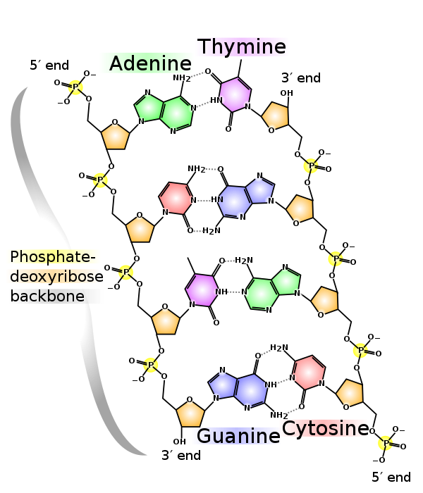
Depending at which level you are looking at this particular molecule, analyzing it can be quite complex. Since we are talking about DNA Sequences it is safe to assume that we want to analyze the sequences of Adenine/Thymine/Guanine/Cytosine nucleotide sequences.

These sequences at the data level looks quite simple as they can be encoded as a series of characters from this set: {'A', 'T', 'G', 'C'}. The arrangement of these characters and their patterns is what leads to life in all of it's complexity.

You can find a sample datasets over here on Kaggle if you want to follow along and play with it a bit!

Finally, the information content of a given DNA structure is closely related to how complex it is. If we had a full DNA snippet that contains only one character (i.e. A) it is safe to assume that this snippet is not complex and doesn't hold much information.

However, a more complex DNA snippet with all characters and different patterns is assumed to hold more information. This is where a complexity measure is important which can quantify this difference!

Kolmogorov Complexity

The Kolmogorov complexity of an object, such as a piece of text, is the length of a shortest computer program (in a predetermined programming language) that produces the object as output. It is a measure of the computational resources needed to specify the object, and is also known as algorithmic complexity. (https://en.wikipedia.org/wiki/Kolmogorov_complexity)

In a nutshell, the kolmogorov (K) complexity is simply the size of the shortest program that can produce the desired object. It's a theoretical measure because the programming language is not defined.

As an example if we had these two strings: abababababababababababababababab and 4c1j5b2p0cv4w1x8rx2y39umgw5q85s7

The first one would have a smaller K complexity because we could write the following pseudo-program write ab 16 times, which is a fairly small program.

The second strings has a higher K complexity because the only obvious way of writing the program would be write 4c1j5b2p0cv4w1x8rx2y39umgw5q85s. which is bigger than the first one.

In practice however, the K complexity is simply approximated using compression algorithm in the following way:

K(object) <= size(Compress(object) + source code of Decompress()

This is practical because we know that a compression algorithm will have a easier time compressing something with very low complexity than something that is highly complex. By taking the size of the whole archive generated by a compression (i.e. something like a .zip file which include the decompressor function) we have a good upper-bound approximation of the K complexity of an object.

For more details on Kolmogorov and a code walk-through do check out this video on the subject:

Now, this is great! We know that we can approximate K complexity by zipping files away. Let's look at how this looks like in an actual research project! 🔬

Kolmogorov Complexity Applied to DNA Sequences

The paper we will be looking at is the following one "Comparison of Complexity Measures for DNA Sequence Analysis", which you can also find on my Github. I'll highlight the important bits and share my interpretation of the result.

This paper looks into DNA analysis by computing and comparing complexity measures, in addition to providing a review of recent studies regarding the measurement of DNA complexity. The authors compare Shannon Entropy, Kolmogorov Complexity (approximated by Lempel-Ziv Compressibility) and statistical complexity, and observe that regions corresponding to genes have consistently different complexity measures (i.e., they are more regular) than those regions that do not have any gene associated with them. This provides insight on how to develop new tools for automated DNA analysis.

The important bits in the abstract is that there are other measure of complexity than K complexity that can be used and that K complexity is approximated using Lempel-Ziv complexity which we'll see in the next section!

Gusev and others evaluate genetic complexity by finding the amount of repetitive sequences (commonly interpreted as regulatory DNA) with a Lempel-Ziv measure [3]. The role of protein coding DNA and regulatory DNA has been understood only recently, and provides insight on the belief that organism complexity is related to the amount of “extra” DNA

Here, it means that K complexity is a good proxy for an organism complexity. Therefore, Lempel-Ziv, which is a good proxy for K complexity, should be also a suitable proxy.

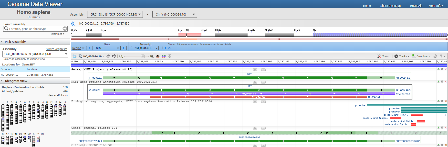
For the purposes of this study, the authors chose a short sequence of genomic data, taken from the generic Human Genome Project, of 384 kbp (kilo base pairs). Specifically, the data corresponds to Chromosome Y [10], [11] (locus NT_011896) from base number 2,781,480 to base number 3,165,480, encompassing three genes.

Their data is all coming from the Human Genome Project. You can browse the Y chromosome right here in the NCBI website if you want.

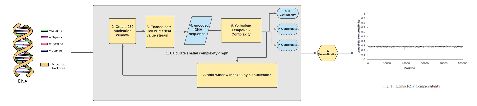
A moving window (local profile) analysis of 250 base pairs per computation was performed, and a graph of the variation of the specified complexity measure along the full sequence was produced.

This means that they used a window of 250 nucleotide to calculate 1 point for a metric of interest (i.e. Lempel-Ziv, Shannon Entropy or statistical complexity).

The analysis window was moved 50 base pairs after each computation, in an overlapping manner.

This means that they calculated 1 metric for a window of 250 nucleotide, then shifted the window to the right by 50 nucleotide, repeated the analysis, so on until the end. This allowed them to then plot all of these complexity metric across the whole length of the Y chromosome and create a sort of spatial-complexity graph.

In this paper they compared 3 type of complexity measures, but we will delve only on Lempel-Ziv.

Kolmogorov Complexity is based on the concept that if a given sequence S can be generated by an algorithm smaller than the length of the given sequence, then its complexity corresponds to the size of the algorithm.

If a sequence is truly complex and random, the shortest representation is the sequence itself [17]. These models were later refined by Chaitin when algorithmic information content was proposed [18]. The issue is that Kolmogorov Complexity itself is not computable.

In the present study, the Lempel-Ziv approximation to Kolmogorov Complexity was used. It quantifies the amount that a message can be compressed using the LempelZiv-Welch algorithm.

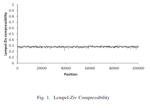
So their whole process was able to produce this graph of spatial-LZ complexity. Let's take a closer look on this metric to understand how to use it ourselves!

Lempel-Ziv Complexity

Lempel-Ziv complexity stem directly from the LZ type of lossless compression algorithm, where the two popular one are LZ77 and LZ78.

Basically, to get LZ complexity you just need to take these algorithm and pop-off the saving of the compressed information (i.e. which in practice is a bit overkill since even with the compression information we get a good upper-bound on the K complexity).

It needs to be noted that LZ complexity works on stream of bits for the compression, so what is imputed needs to be a sequences of 0s and 1s.

LZ-77 works roughly as follows given a stream of bits read from left to right do the following:

1. Read first bits.
2. Put in exhaustive memory or not (if pattern already seen).
3. Find maximum component from exhaustive memory to explain the data appearing on the right.
4. Put new component inside exhaustive memory when streak is broken.
5. Complexity = |{Exhaustive Memory}|

If you wanted to compress then you would use that exhaustive memory, but for calculating complexity you don't really need to keep that info.

A simple Python implementation of LZ complexity would look like this (all credit to the user Nareen on Github):

It's a fairly short algorithm and in this particular implementation, the sub strings generated are actually kept so you can print them out if you are curious!

For more details on Lempel-Ziv complexity, feel free to check out the following tutorial or check this cool Github Project:

Now that we know how Lempel-Ziv works and that we know it's used directly with DNA sequences, we can bridge the two bits of knowledge together to create our data pipeline!

Data Pipeline for Complexity Analysis

With the information now in hand we can craft a good data pipeline in which we understand clearly each components that compose it. We will follow the previously mentioned conference paper so as to generate a similar looking spatial-complexity graph.

Let's break down each components after we have loaded a DNA sequence of raw ATGC characters into our code:

1. The main part of our code has to do with calculating the spatial complexity graph. To do so we will need to repeat an analysis that will calculate multiple K complexity metric across the length of the DNA sequence.
2. The first step in this loop is to create a 250 nucleotide window where we are at in the DNA sequence.
3. We then encode this window of 250 nucleotide into a sequence of bits. We do this simply by converting the characters into their bits representation.
4. What we get out of this is a series of 0s and 1s representing a 250 nucleotide sub-sequence.
5. We then feed that series of 0s and 1s into our code we've seen earlier that calculate the LZ complexity.
6. What we got out of from an binarized input of 250 nucleotide is one metric that determine the K complexity of that snippet. We store that information.
7. We then shift the start and end index of our window by 50 nucleotide to the right. This will loop back at the start of our data pipeline loop.
8. Once we've run through the full length of the sequence we normalize the K complexity series we've created to see how it differs across the DNA sequences!

The pipeline is pretty simple in order to get the data from it's raw ATGC format into a complexity metric graph. Let's tie this into some very basic Python code and show how to produce a similar kind of graphs we've seen earlier! ✅

DNA Complexity Analysis in Python

Once the whole data pipeline is mapped out, it's pretty simple to construct a working analysis without too much trouble. There are always optimization that can be done, but I like to start my analysis with a easy to understand state and then optimize afterward for performance.

You can find the full code over here on my Github btw!

Loading the Data

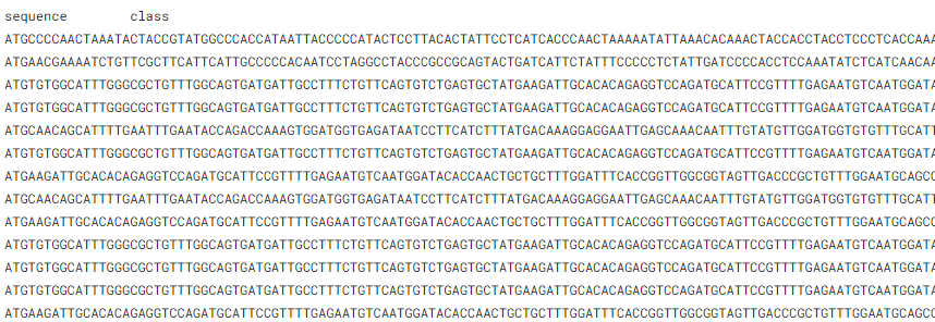
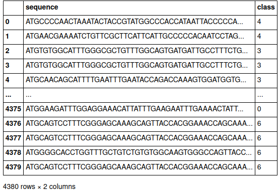
The very first step is to read and load the data from Kaggle into a pandas data frame, it's the easiest way to read CSV in my opinion.

We get the following data frame:

Creating the Helper Functions (i.e. the yellow boxes in the image)

Now it's time to define all of the yellow boxes in our diagram. Usually, when you plan a research analysis and when you code it you will see that some of the boxes that were well delimited kind of blend better together as one.

It's all right to not follow exactly the plan, the purpose is just to create a proper mental model before coding so that you know what to aim for and not get too lost!

Here we have multiple important helper functions:

1. the complexity code which we already seen in the previous section.
2. the string-to-binary converter which is needed to "translate" our ATGC sequence into something digestible for the complexity code.
3. the window generator which role is purely to slice a given data sequence. Here I've used a generator, but I could have just used a for loop.
4. a helper function to generate a list of LZ complexity metric, which leverage the window generator and the rest of the helper functions.
5. a simple normalizer functions to mimic what the paper has done.
6. finally a helper function to re-create the complexity plot using matplotlib!

None of that is optimized of course as I'm using lists like time is no object. 👴👴👴👴

Stitching the analysis together!

Finally, by creating all of our small helper functions we are able to stitch them together very easily!

To simplify the analysis we've glued together all of the sequences in the pandas data frame to create a "pseudo chromosome".

I'm not too sure what the row in the data frame are exactly, but for teaching purpose let's assume that this is actually a sliced up chromosome that we are stitching back together.

Now we are able to generate cute picture of complexity at different "resolution" to see how different is the spatial complexity along the fake chromosome we've built!

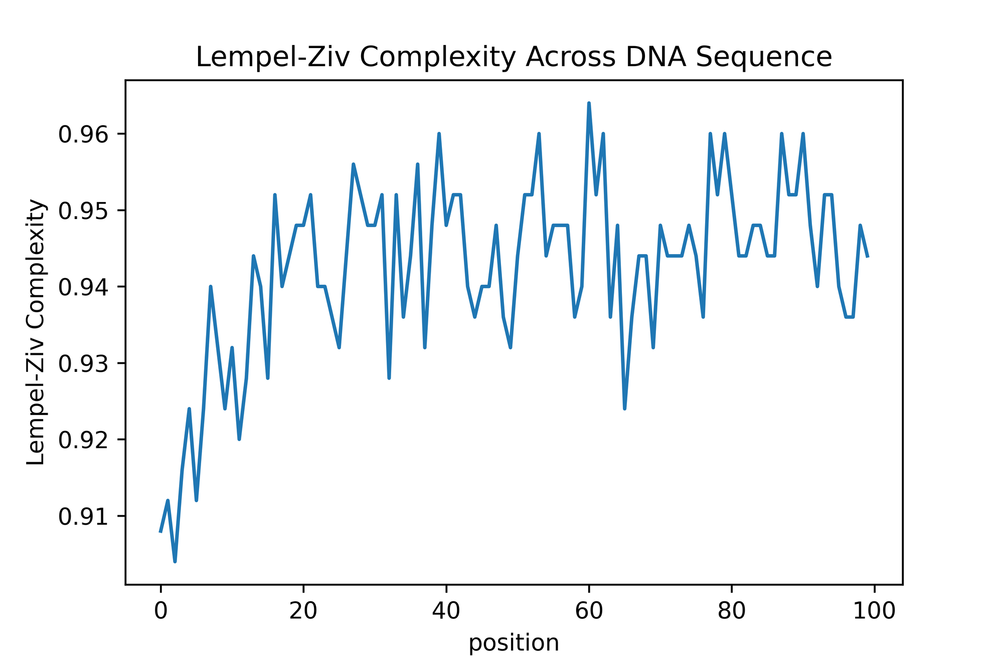
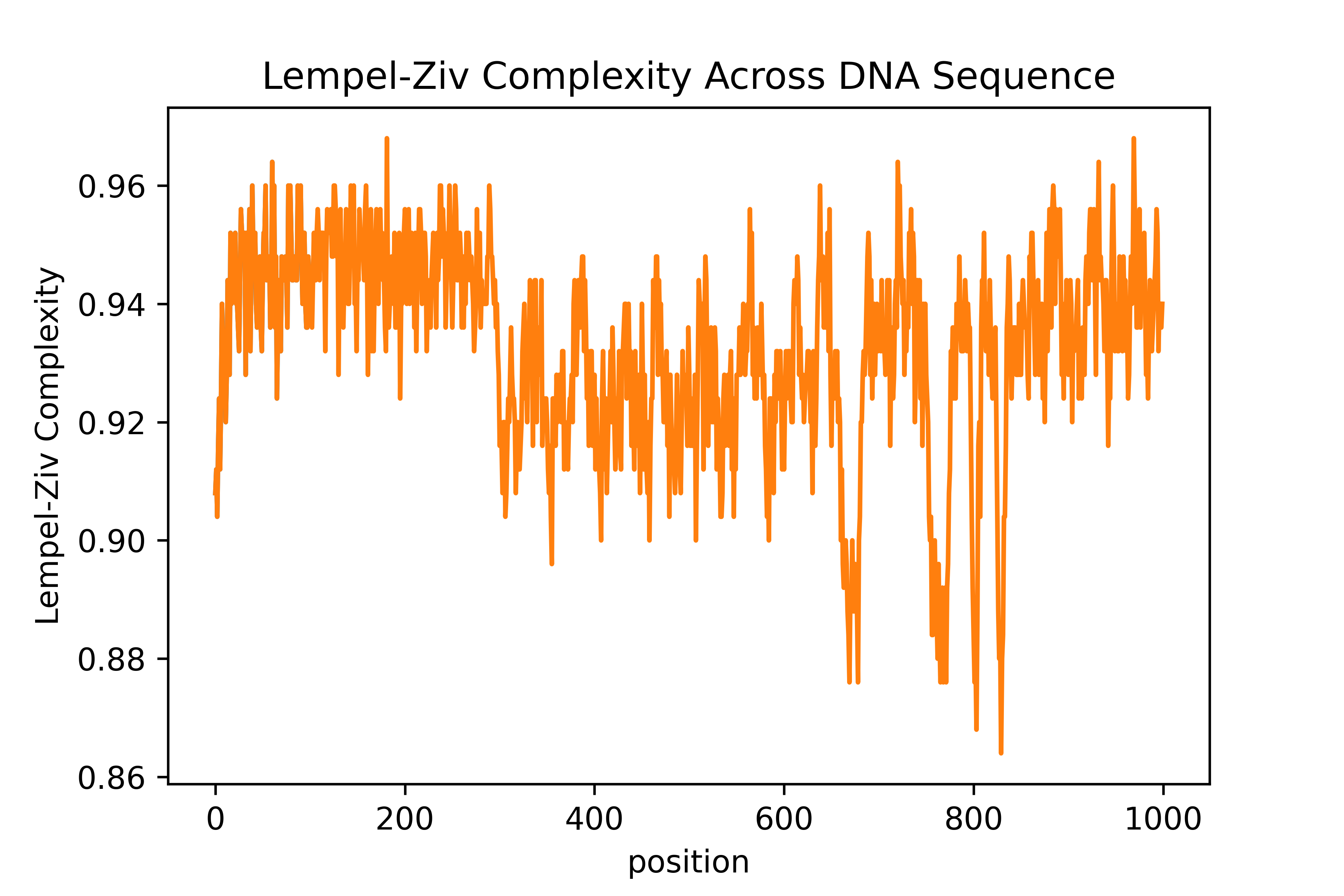
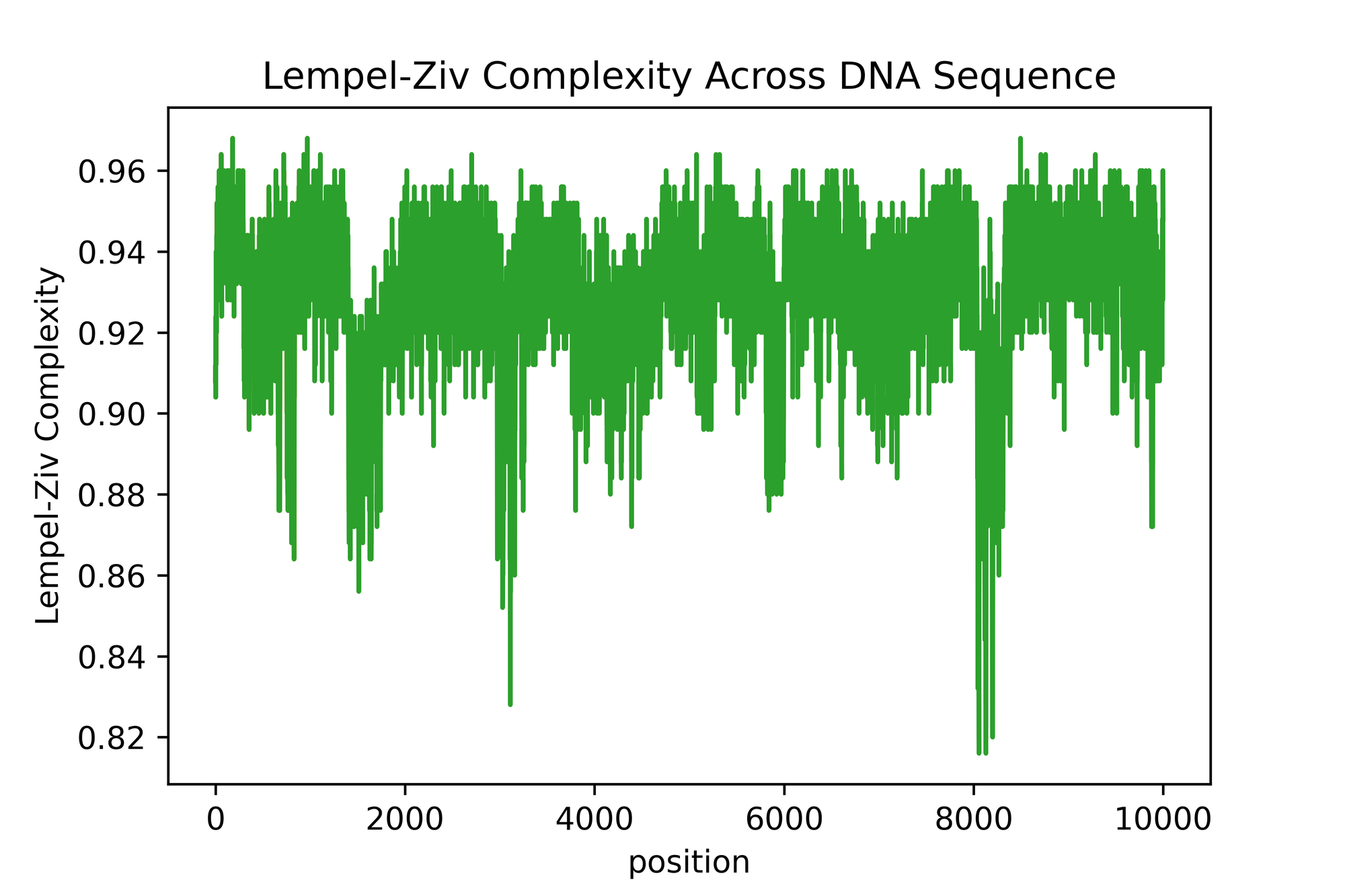
The output graph looks somewhat similar to what is in the paper! However, there is many difference in the sense that I feel that the normalization here isn't exactly the same as the one they used. It's a bit difficult and opaque to know exactly what they did, but that's what happen when you publish a research paper without code 😤😤😤

There is segment which are relatively way less complex than other in this stitched up sequence. This seems to make biological sense. However, we can't know if the dips we are seeing are any significant since we have no control (i.e. a randomized DNA sequence which is pure synthetic gibberish).

For demonstration purpose, we were able to go through the full motion pretty well! So, that's it! This is how we are able to use Kolmogorov complexity to analyze DNA sequences using Python! 😊

Conclusion

To conclude, K complexity and it's applications are a very handy toolset to have at your disposal, especially in the life science context. Being able to take two recording, participants or cohorts and be able to put a quantity on the complexity difference while doing the comparison is very useful.

It allows you to enrich your analysis with a intuitive layer of understanding while at the same time veering off qualitative characterization like : "look at these two plots, the first one looks simpler than the second one!".

However, before we close this article let's look at the conclusion of the article mentioned in the earlier section:

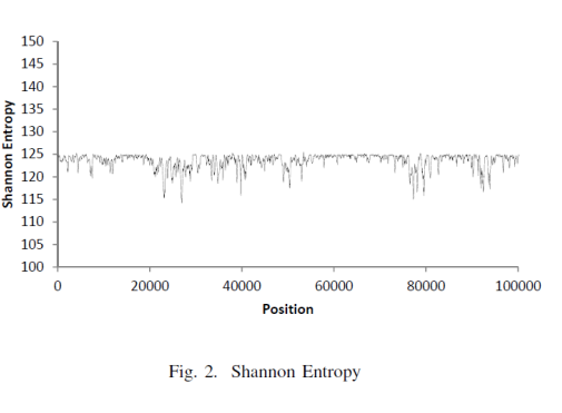
The authors showed these graph for LZ and SE and concluded the following 👇

The Lempel-Ziv compressibility measure only shows that DNA sequences can be generated by a deterministic process, but it cannot distinguish between coding and non-coding DNA.
[...]
The average compressibility measure for the data analyzed is similar to the average compressibility measure for random data, thus indicating that the Lempel-Ziv measure analyzes algorithmic content, not information.
[...]
A second interesting aspect of the study conducted is the relationship between complexity and information content. The complexity measures that were not based on information content do not provide much information for further analysis

This is a very good example of why knowing only one metric is quite dangerous. It can, in some instance, blind you. Being able to run your analysis with multiple type of metric allows you to get a clearer picture of the process your are analyzing.

In this specific instance, the LZ complexity metric was as good as compressing coding/non-coding sequences. Similarly, random DNA sequences weren't much different in size once compressed. This can means multiple things, but it's always very important to keep in mind where the metric is coming from when using it.

So as a closing word, be extra-careful with the interpretation of your analysis and always diversify your toolset when it comes to bioinformatics!

---

If you have a questions or comment, don't hesitate to shoot me a email at mail@yacinemahdid.com! Also, if you liked the content don't hesitate to subscribe to the newsletter!  

👋