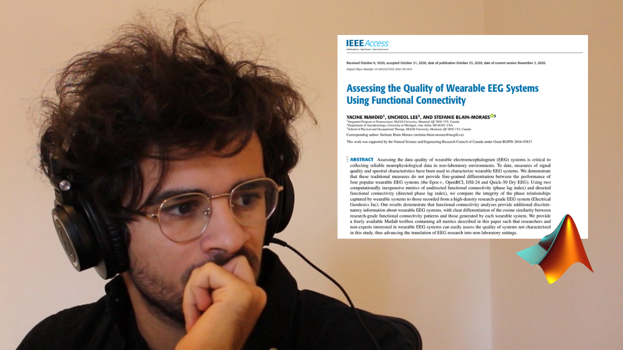
Reproducing my own research paper after a year and a half of publishing!
A year and a half ago I've published a paper using some code I've created! In this blog post I've checked out if I would be able to reproduce it easily!
My very first real software that I've made back in University was a pretty hard core one. I was fresh out of COMP 202 Foundations of Programming at McGill and I wanted to fast-track my learning by helping out in a research lab.
I was able to get a credited research project to develop an application that given Electroencephalographic data could output a bunch of metrics that was useful for computational neuroscientist.
The project was a lot to take on as it involved:
- MATLAB a programming language I wasn't familiar with.
- Building a graphical user interface, which I had no idea how to build.
- Coding quite a few analysis techniques that I've never heard before (like Symbolic Transfer Entropy and Weighted Phase Lag Index).
- Piping data so as to create repeatable analysis.
- Saving application state and more generally dealing with users inputs.
I've honestly learned a lot from this and it really pushed me to deliver on a tight schedule! Now, you can image that such an app made by a undergraduate fresh out of his first coding class wouldn't be top quality. I kept working on it for almost all of my time in Academia.
I went on to refine it over and over until I could use the software in most of my analysis. This lead me to create an internal library that allowed me to be very productive in my research!
It's research code, so it's far from perfect or very useable. However, it still has the merit of being somewhat easy to reproduce research results!
So I built the thing, published a paper using the analysis and then got the following question after a year and a half asking me help to reproduce the results 👇👇👇
Question
Dear Prof Mahdid,
starting from the beginning, I would like to reproduce with EEGApp the results that are presented on https://ieeexplore.ieee.org/stamp/stamp.jsp?tp=&arnumber=9237931.
In particular, for example, I would like to obtain Figure 4 (PLI and dPLI) of the paper, performing functional connectivity analysis with EEGApp on egi headseat data (shared on gitub).
I used egi_open data.
As parameters Length of analysis segment (10s), number of permutations (20), pvalue (0.05) and bandpass alpha.
But the results are not the same of the paper.
Can you please ask you to explain the steps that I need to perform to obtain the results of Figure 4, for example?
In addition, I tried to perform graph analysis on egi_open data and emotiv_open data shared on
https://github.com/BIAPT/Assessing-the-Quality-of-Wearable-EEG-Systems-Using-Functional-Connectivity. The egi data seems to give a graph theory result but emotiv_open not.
Is it possible to compare graph theory analysis in open and closed conditions in egi and emotiv?
My final scope is to test the EEGApp and then apply it on my Epoc and Flex data.
thanks
This question has a lot of component that are mixed together because the code and the paper aren't clear enough about how to reproduce the result. This is my bad, I should have taken more time to explain the practical technical details of the analysis.
So, in this blogpost I'll dive in a codebase I haven't touched since March 18 2020, which is about 2 decades ago in software engineering, and reproduce the result of my paper!
Overview of the Codebases
The code mentioned in the question is split into 3 different codebase, which at that time make sense (I still think it does, but it sure complicate a lot the reproduction of the paper). Two of the codebase are important, the other one is deprecated as it isn't that easy to use.
EEGapp 🧠(not much used anymore)
EEGapp contains a very early version of the analysis that were used in my paper along with a GUI. The paper was initially written using the output of me clicking on the GUI to configure the pipeline. However, I quickly realized that this was very cumbersome and wasting a lot of my time. Most of things I had to fight and debug were things related to the GUI, not the analysis.
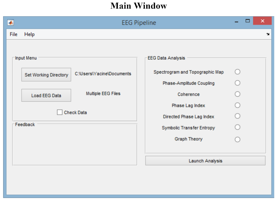
(props to all engineers working on GUI/Frontend, this thing is hard!)
Therefore, I started to rip out the analysis out of the GUI and use only the library that powered the software. At some point it made absolutely no sense to keep using the GUI so I've created scripts using the library and shared that with my lab.
This was the basis of NeuroAlgo.
NeuroAlgo 🖥️
This codebase was created much later in my research career when I was doing my Master and PhD at McGill. I've matured a bit in term of software development, but I still wasn't a top-notch programmer.
It's lightweight and somewhat easy to use. I had lots of good ideas for improvement , but tinkering with a library isn't in and of itself very worthwhile in Academia.
Still, it allowed our whole lab to have all analysis share a common language and core. This library was usually downloaded and imported into each of the other analysis that my lab wanted to use and this paper makes heavy use of it.
Paper Codebase 📝
The codebase for my paper titled "Assessing the Quality of Wearable EEG Systems Using Functional Connectivity" is using NeuroAlgo in order to analyze the data I've gathered (it's my brain btw)! It simply a collection of scripts that uses all of the analysis techniques and the functionalities I've coded in NeuroAlgo in order to generate the figures and numbers!
It's fairly straightforward to use, but it requires to have both the NeuroAlgo library and the Paper codebase at hand to run the analysis. In retrospect I could have included the NeuroAlgo library straight into a lib section of some sort to avoid the issue of backward compatibility 😕😕😕
Now that we know how we roughly shaped the codebases we can dive into the details of answering this researcher lost in the mess I've created.
Breaking Down the Question
Let's break down the question into small chunks and answer each bits.
starting from the beginning, I would like to reproduce with EEGApp the results that are presented on https://ieeexplore.ieee.org/stamp/stamp.jsp?tp=&arnumber=9237931.
This is the first issue. At the point where I published the article, I've decided to move the analysis to NeuroAlgo as I had much more flexibility and results were easier to reproduce! Therefore, it's not EEGapp that we should focus on it's NeuroAlgo!
In particular, for example, I would like to obtain Figure 4 (PLI and dPLI) of the paper, performing functional connectivity analysis with EEGApp on egi headseat data (shared on gitub).
I used egi_open data.
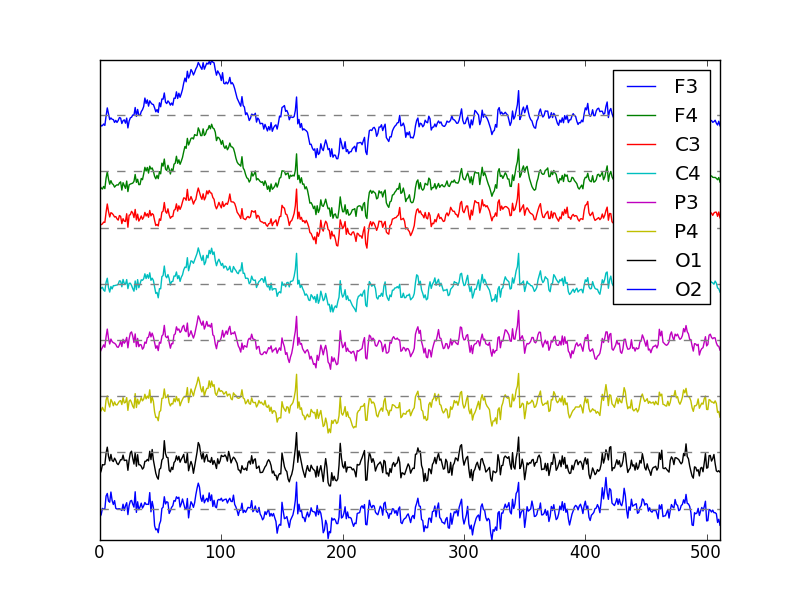
So the very first part is to reproduce this figure:
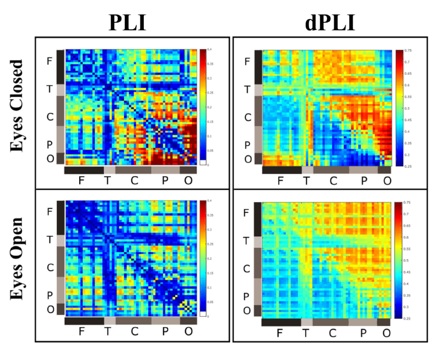
The exact formatting of the figure cannot be reproduced because I've used Inkscape and manually created them. However, the jet-colored matrices are reproducible "easily" with the code provided. We'll dive into the rest of the question before showing how to reproduce the analysis.
As parameters Length of analysis segment (10s), number of permutations (20), pvalue (0.05) and bandpass alpha.
But the results are not the same of the paper.
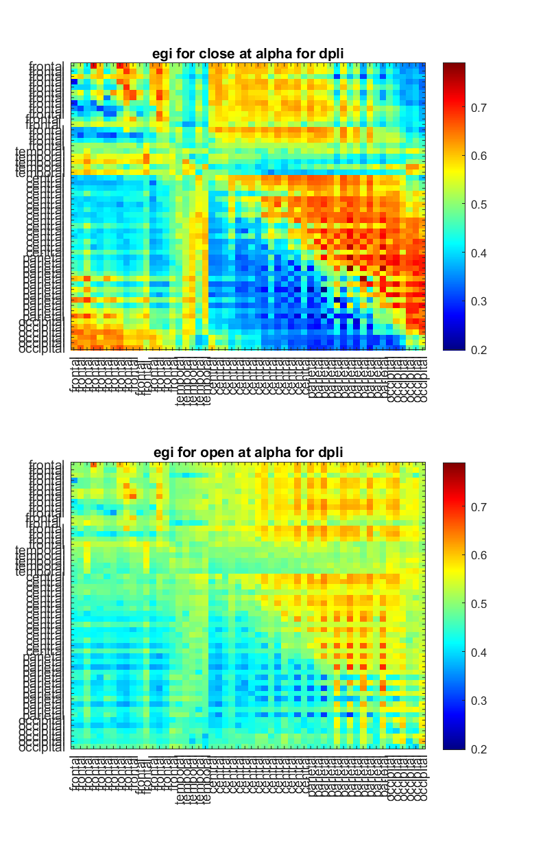
Here what happen is most likely that the author used the `egi_open.set` file that I've provided with the code and feed it into EEGapp. This is will not yield the same figure as shown above even thought the analysis is similar because there are a few cosmetic change that were done in order to make the image more understandable:
- Channels were ordered in frontal, temporal, central, parietal and occipital region.
- The range of the colormap was thresholded in order to be similar to the other matrices to be able to compare.
These two change will give very different pattern!
In addition, I tried to perform graph analysis on egi_open data and emotiv_open data shared on
https://github.com/BIAPT/Assessing-the-Quality-of-Wearable-EEG-Systems-Using-Functional-Connectivity. The egi data seems to give a graph theory result but emotiv_open not.
Is it possible to compare graph theory analysis in open and closed conditions in egi and emotiv?
For the graph theory result, if you are using EEGapp it's very cumbersome. There are multiple things internal to how the .set file work that can break in the EEGapp version of the graph theory analysis (like the location data structure being present or not).
Also, the way I coded the graph theory segment in EEGapp forces you to use a very strict way of creating a graph. This bias lead to analysis that aren't as rich as they could.
In the NeuroAlgo library I've decoupled a lot of things so then it's possible to simply mix and match different part of the analysis in order to use graph theory. One example workflow would be to:
- calculate PLI, wPLI or STE with the parameters of your choice to create a matrix of connectivity.
- threshold the matrix using the utility function.
- then use one of the many graph theory measure available to get a metric.
This mix and matching allow you to get more robust analysis without just dealing with a black box!
My final scope is to test the EEGApp and then apply it on my Epoc and Flex data.
If this is the case you are much better off to use NeuroAlgo and script your analysis yourself!
Anatomy of a NeuroAlgo Script
Before diving into the whole reproduction of the paper I want to take the time to put some emphasis on why scripting is much better than clicking around in a GUI and show you how it looks like.
With a GUI, you have no way but to click away in order to generate the output. Recording what you clicked on is error prone and there is a lot of things that can go wrong when someone else need to reproduce your work. If you omit to say something very basic you clicked on to generate an result, this might lead a beginner to get completely lost.
A script has a higher barrier of entry than a GUI for sure. However, once the script has been demystified, it is much more easy to use. It's basically a text that if written well doesn't have much complexity in it and is 100% reproducible because it's the same script that someone else ran (~90% reproducible in fact if the environment you ran the code on isn't part of the script).
Here is an `example_analysis.m` that I've baked into my NeuroAlgo library so that people can familiarize themselves with the syntax:
%% Loading a .set file
% This will allow to load a .set file into a format that is amenable to analysis
% The first argument is the name of the .set you want to load and the
% second argument is the path of the folder containing that .set file
% Here I'm getting it programmatically because my path and your path will
% be different.
[filepath,name,ext] = fileparts(mfilename('fullpath'));
test_data_path = strcat(filepath,filesep,'test_data');
recording = load_set('test_data.set',test_data_path);
%{
    The recording class is structured as follow:
    recording.data = an (channels, timepoints) matrix corresponding to the EEG
    recording.length_recoding = length in timepoints of recording
    recording.sampling_rate = sampling frequency of the recording
    recording.number_channels = number of channels in the recording
    recording.channels_location = structure containing all the data of the channels (i.e. labels and location in 3d space)
    recording.creation_data = timestamp in UNIX format of when this class was created
%}

%% Running the analysis
%{
    Currently we have the following 7 features that are usable with the
    recording class: wpli, dpli, hub location, permutation entropy, phase
    amplitude coupling, spectral power ratio, topographic distribution.
    If you want to get access to the features that are used without the
    recording class take a look at the /source folder
%}

% Spectral Power
window_size = 10;
time_bandwith_product = 2;
number_tapers = 3;
step_size = 0.1; % in seconds
bandpass = [8 13];

result_sp = na_spectral_power(recording, window_size, time_bandwith_product, number_tapers, bandpass,step_size);

% wPLI
frequency_band = [7 13]; % This is in Hz
window_size = 10; % This is in seconds and will be how we chunk the whole dataset
number_surrogate = 20; % Number of surrogate wPLI to create
p_value = 0.05; % the p value to make our test on
step_size = window_size;
result_wpli = na_wpli(recording, frequency_band, window_size, step_size, number_surrogate, p_value);

% dPLI
frequency_band = [7 13]; % This is in Hz
window_size = 10; % This is in seconds and will be how we chunk the whole dataset
number_surrogate = 1; % Number of surrogate wPLI to create
p_value = 0.05; % the p value to make our test on
step_size = window_size;
% as of July 2021 the dPLI code was corrected. Please use na_dpli_corrected
result_dpli = na_dpli_corrected(recording, frequency_band, window_size, step_size, number_surrogate, p_value);

% Hub Location (HL)
frequency_band = [7 13]; % This is in Hz
window_size = 10; % This is in seconds and will be how we chunk the whole dataset
number_surrogate = 10; % Number of surrogate wPLI to create
p_value = 0.05; % the p value to make our test on
threshold = 0.10; % This is the threshold at which we binarize the graph
step_size = 10;
a_degree = 1.0;
a_bc = 0.0;
result_hl = na_hub_location(recording, frequency_band, window_size, step_size, number_surrogate, p_value, threshold, a_degree, a_bc);

% Permutation Entropy (PE)
frequency_band = [7 13]; % This is in Hz
window_size = 10; % This is in seconds and will be how we chunk the whole dataset
embedding_dimension = 5;
time_lag = 4;
step_size = 10;
result_pe = na_permutation_entropy(recording, frequency_band, window_size , step_size, embedding_dimension, time_lag);

% Phase Amplitude Coupling (PAC)
window_size = 10;
low_frequency_bandwith =[0.1 1];
high_frequency_bandwith = [8 13];
number_bins = 18;
step_size = 10;
result_pac = na_phase_amplitude_coupling(recording, window_size, step_size, low_frequency_bandwith, high_frequency_bandwith, number_bins);

% Spectral Power Ratio (SPR)
window_size = 10;
time_bandwith_product = 2;
number_tapers = 3;
spectrum_window_size = 3; % in seconds
step_size = 5; % in seconds
result_spr = na_spectral_power_ratio(recording, window_size, time_bandwith_product, number_tapers, spectrum_window_size, step_size);

% Topographic Distribution (TD)
window_size = 10; % in seconds
step_size = window_size; % in seconds
bandpass = [8 13]; % in Hz
result_td = na_topographic_distribution(recording, window_size, step_size, bandpass);

% Note: You can put the value you want directly into the function call,
% I've laid them out beforehand so that you understand what each value
% means
If this looks scary to you, don't worry. I'll break it down so that it makes a bit more sense. Most of the code here is just comment that is there for documentation purpose.
Loading data
[filepath,name,ext] = fileparts(mfilename('fullpath'));
test_data_path = strcat(filepath,filesep,'test_data');
recording = load_set('test_data.set',test_data_path);
In NeuroAlgo, the format that is accepted for EEG data is the .set file. Why? Because it was the format I used in my lab. The way to load a file is just to grab it's path and the name of the file and call the load_set function!
The load_set function isn't black magic. You can take a look at it directly in the repository! Most of the code that handle the data actually leverage code from other library that are much more robust than mine!
Running an Analysis
Running an analysis in NeuroAlgo is pretty straightforward because it's always the same thing. You set up your parameters, give the input file to work with and the parameters. Then you get the result and you use that for future analysis if needed.
Here is an example with spectral power:
% Spectral Power
window_size = 10;
time_bandwith_product = 2;
number_tapers = 3;
step_size = 0.1; % in seconds
bandpass = [8 13];

result_sp = na_spectral_power(recording, window_size, time_bandwith_product, number_tapers, bandpass,step_size);
That's it. The complexity of how spectral power is calculated is just abstracted into the na_spectral_power function (which you can also peak into if needed)! It's the same syntax for each of the analysis technique.
The result data structure contains the actual output of the function, but also all the meta data that generate it. This way, the ouput always has the recipe that produced it attached to it!
Now that this is more clear, we can go ahead and try to reproduce my paper!
Setting Up Everything 🛠️
There is a few things you will need in order to generate the figure/result for this paper. Let's walk through the steps!
Get MATLAB
First off, you need to have MATLAB installed. If you do have an academic license, install that up following the MATLAB documentation!
Watch out for the version of MATLAB that you need to reproduce a paper. Different version of MATLAB can behave slightly differently and sometime be backward incompatible. In my case for that paper I've used MATLAB2019b so get that.
Install MATLAB add-ons
The MATLAB ecosystem makes use of add-ons to augment the capability of the core-software. You need to get three of them in order for NeuroAlgo to work (and by extension the code to reproduce the article).
- Signal Processing toolbox
- Statistics and Machine Learning Toolbox
- Symbolic Math Toolbox
Once you downloaded all of them, reboot your MATLAB setup for the next step!
Clone the Repositories
The two codebase you want to get is:
It's very important to always try to take the version that was used while making the paper as it isn't guaranteed that it will be backward compatible. Even more so if it's non-professional software engineers that made the codebase, like I did!
The final steps of the setup is to add everything to the MATLAB path (both codebase) by just right clicking and selecting "add to path > Selected Folder and Sub Folders"
Testing the Setup
To ensure that everything run smoothly on the NeuroAlgo side, do run the example_analysis.m file in the library! This will run all available analysis on the test_data.set file which contains a short test data EEG recording. Once you know that it's working, you can then go ahead and move to the other repository where the analysis is actually at.
Reproducing the Analysis
I've tried to make it as easy as possible to reproduce my code for the paper. Basically it all came down to generating the features needed for the analysis and then creating the figure based on the results.
This was bundled into two scripts that you should run one after the other:
calculate_features.mgenerate_figures.m
Basically what it will do is generate all of the feature needed for the paper in the first run with the first script and store that locally. Then it will generate figures which are the one you can see in the paper!
All of the data is located in the repository since they are fairly small and fitted in the Github size limit (/data folder)!
and that's it!
The only file you really need to dig through to understand what is going on is the one that is calculating the features! The figure one is mostly to just ensure that we can generate the edit ready picture for the paper!
%% General Parameters
DATA_DIR = "/home/yacine/Documents/Assessing-the-Quality-of-Wearable-EEG-Systems-Using-Functional-Connectivity/data/";
OUT_DIR = "/home/yacine/Documents/Assessing-the-Quality-of-Wearable-EEG-Systems-Using-Functional-Connectivity/result/";

STATES = {'closed','open'};
HEADSETS = {'egi','quick_30','dsi','open_bci','emotiv'};
FREQUENCIES = {'alpha', 'beta', 'theta', 'delta'};

%% Experimental Parameters
% Spectral Power
SP = struct();
SP.TBP = 2;
SP.NUM_TAPER = 3;
SP.SPR_WINDOW_SIZE = 2; % in seconds
SP.STEP_SIZE = 0.1; % in seconds
SP.BP = [1 30];

% Topographic Distribution
TD = struct();
TD.BP = [8 13]; % in Hz

% wPLI and dPLI
PLI = struct();
PLI.BP = [8 13]; % This is in Hz
PLI.WINDOW_SIZE = 10; % This is in seconds and will be how we chunk the whole dataset
PLI.NUMBER_SURROGATE = 20; % Number of surrogate wPLI to create
PLI.P_VALUE = 0.05; % the p value to make our test on
PLI.STEP_SIZE = PLI.WINDOW_SIZE;


for f = 1:length(FREQUENCIES)
    frequency = FREQUENCIES{f};
    bandpass = [];
    switch frequency
        case "alpha"
            bandpass = [8 13];
        case "beta"
            bandpass = [13 30];
        case "theta"
            bandpass = [4 8];
        case "delta"
            bandpass = [1 4];
        otherwise
            disp("Wrong frequency!")
            return
    end
    for h = 1:length(HEADSETS)
        headset = HEADSETS{h};
        for s = 1:length(STATES)
            state = STATES{s};

            out_filename = strcat(OUT_DIR, frequency,filesep, headset,"_",state,".mat");
            result = struct();

            disp(strcat("Analyzing ", headset , " At state: ", state));
            filename = strcat(DATA_DIR, headset, filesep, headset, "_", state, ".mat");
            recording = load_mat(filename);

            % Spectral Power

            SP.window_size = floor(recording.length_recording/recording.sampling_rate); %dynamic parameter

            result.sp = na_spectral_power(recording, SP.window_size, SP.TBP, ...
                                SP.NUM_TAPER, SP.SPR_WINDOW_SIZE, SP.BP, SP.STEP_SIZE);

            % Power Topographic Map
            TD.window_size = SP.window_size; % dynamic parameter
            TD.step_size = SP.window_size;
            TD.BP = bandpass;
            result.td = na_topographic_distribution(recording, TD.window_size, ...
                                                    TD.step_size, TD.BP);

            % Functional Connectivity
            PLI.BP = bandpass;
            result.wpli = na_wpli(recording, PLI.BP, PLI.WINDOW_SIZE, PLI.STEP_SIZE, ...
                                  PLI.NUMBER_SURROGATE, PLI.P_VALUE);

            result.dpli = na_dpli(recording, PLI.BP, PLI.WINDOW_SIZE, PLI.STEP_SIZE, ...
                                  PLI.NUMBER_SURROGATE, PLI.P_VALUE);


            % If we are not working with the egi headset we should also load
            % the downsampled egi headset
            if strcmp(headset, "egi") == 0
               disp(strcat("Calculating functional connectivity on the downsampled ", headset));
               filename = strcat(DATA_DIR, headset, filesep, "egix",headset, "_", state, ".mat");
               recording = load_mat(filename);

               result.down_sampled_wpli = na_wpli(recording, PLI.BP, PLI.WINDOW_SIZE, PLI.STEP_SIZE, ...
                                  PLI.NUMBER_SURROGATE, PLI.P_VALUE);
               result.down_sampled_dpli = na_dpli(recording, PLI.BP, PLI.WINDOW_SIZE, PLI.STEP_SIZE, ...
                                  PLI.NUMBER_SURROGATE, PLI.P_VALUE);
            end


            % Save the data
            save(out_filename, '-struct', 'result');

        end
    end
end
The code is not too long, it's about 100 lines of code and is making heavy use of NeuroAlgo by using the scripting syntax I've mentioned earlier! 😃
I'm looping through the analysis multiple time because I'm calculating the same metric over different bandpass in the EEG data.
Conclusion
I hope that was useful! Don't hesitate if you have any more question, but I've tried my best to make something that I could use for myself again and again throughout my research!
It's not the best documented codebase and there is a lot of work that could still be done to make it better, however it served me well during my time in Academia!
If you have a questions or comment, don't hesitate to shoot me a email at mail@yacinemahdid.com! Also, if you liked the content don't hesitate to subscribe to the newsletter!