Some concepts in machine learning may at first glance look extremely opaque and difficult to grasp. Yet, most are pretty accessible and simple.

However, they are usually clouded by terminology you don't understand or heavy math notations. When you are faced with one such concept that is stumping you:

1. remember that mathematical notations are just a way to codify the concept. Take your time and translate the math into words.
2. know that there is always a logical flow that you can piece out, draw the concept out or visualize how the component interacts.

In this issue of deep dive in machine learning, we will apply these two tips on the concept of gradient descent.

Gradient Descent Explained

Gradient based optimizers are ubiquitous in machine learning. They are used in deep learning model to find the right set of parameters in order to train a neural network.

Let's try to build the concept of gradient descent from the very beginning!

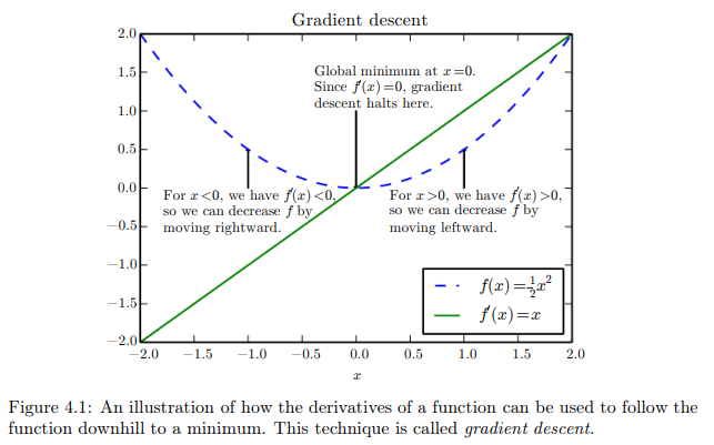
In an optimization problem, we usually wants to minimize a cost function f(x) by changing x.

Taking the derivative of f(x) gives us the slope of f(x) at a point x.

This tells us how changing the input by a bit change the output via this formula:

f(x + e) ≈ f(x) + ef’(x)

Therefore, to minimize f(x) we can take small enough steps in the opposite sign of the derivative.

This is single variable gradient descent in a nutshell.

Taking the derivative of f(x) work when we have a single input variable, but in machine learning you usually have multiple input/features.

To take that into consideration, we use partial derivatives to measures how the function f changes when we modify only the variable x_i at point x.

A gradient is therefore defined as the vector/array containing all the partial derivative of the function f.

Gradient descent in that context has the same essence as in the single variable example, we just need to take a small enough step in the opposite direction of the gradient to minimize f(x).

new_x = x - learning_rate * gradient_f(x)

where the learning rate is just the size of the step we are willing to take in the opposite side of the gradient.

This core is used in many different optimization algorithm like ADAM, Adadelta, stochastic gradient descent, nesterov, etc.

Gradient Descent Visualized

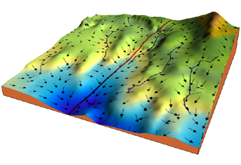
An image is worth a thousand words. If we take this visualization by Jack McKew, we get a deep understanding of how this optimization is occuring:

The mountain is the function we are minimizing (a pretty complex one).

Imagine yourself on that moutain, your position defined by the coordinates.

Gradient descent is simply pulling on your position on that mountain, acting a bit like gravity.

You follow the pull of gradient descent by always taking a step with your legs with a constant stride.

The size of the stride is solely defined by the length of your legs (learning rate).

Once you find a spot where you can't go down anymore you stop!

More Resource

I hope these explanation were useful 😅! If you need more perspective on the subject check out these two ressource:

• A very good in-depth article I recommend on the subject is this one at https://ruder.io/optimizing-gradient-descent/index.html
• Otherwise, do check out the Chapter 4 of the Deep Learning Book for a full summary!

---

Don't hesitate to send me an email at mail@yacinemahdid.com if you have questions! 👋

Yacine